Making a Chip Fall Out of the Workload
OpenAI and Broadcom's Jalapeño is laid out differently from every other flagship accelerator, and OpenAI says it beats NVIDIA at single-user latency. Nobody outside the company has seen the design. I wanted to know if you need to. If the workload forces the architecture, a chip optimized from scratch for the same workload, without looking at theirs, should end up somewhere similar. So I built a simulator, ran a blind search over a few thousand designs, spent most of the project trying to break the results, and ended up writing Verilog. Most of what I believed going in was wrong. One result held.
The best public analysis of this chip is zartbot's teardown, which works from die photos and area accounting. It is the main outside source for everything below. I come at the same chip from the workload side. Read both.
Repo: jalepeno-sim · every number in this piece comes from a committed result file or a cited public source. The markers say what kind of claim each one is: PUBLIC FACT EXTERNAL INFERENCE MY MODEL RTL RESULT
01 What OpenAI disclosed
In June 2026, OpenAI and Broadcom announced a chip called Jalapeño, and at Hot Chips they showed some of it. The headline numbers are large and not very informative: PUBLIC FACT 13.4 petaflops, 216 GB of memory at 15.4 TB/s, 700 watts.1 Every flagship accelerator has numbers like that.
The interesting part is the organization. Most flagship accelerators are built like GPUs: one big shared pool of memory, big caches, huge matrix engines, everything sized for throughput. PUBLIC FACT Jalapeño is described as the opposite on nearly every axis: many small compute "slices," each with its own private slab of memory, no big shared hierarchy, and software deciding where every tensor lives. OpenAI's talk named the things it was avoiding: "contended unified memory subsystems" and "expensive global memory fences."2
OpenAI's published benchmarks claim 1.7x lower latency and 1.9x better tokens per watt than NVIDIA's best. PUBLIC FACT Those are vendor numbers, but they are specific enough to check against.
zartbot's teardown3 argues that architecture determines end-to-end latency: the floor on how fast a token can arrive is set by the shape of the machine, and kernel work cannot move it. On their reading, this machine's shape was chosen for that floor.
Between the Hot Chips talk and the teardown, the public picture is more detailed than you might expect:
1.70 GHz shipping silicon with a plan for 1.80. TSMC 3 nm, one reticle-sized compute die, six HBM4 modules on the package. No big shared cache. Software places every tensor; the KV cache never leaves its slice. A dedicated low-latency network exists just for collective operations, separate from the general one.
The fabric: 128 chips talking at 600 GB/s each in a rack domain, 2,048 chips at 200 GB/s in a pod, over Ethernet on Broadcom Tomahawk 6. And the process story: parts of the chip were designed by their own models writing hardware description code; they claim an AI-designed BF16 multiplier 56% faster at 10% less area, and roughly nine months from RTL to tapeout, versus an industry-typical two to three years.
zartbot's estimates from die shots and area accounting: about 64 slices, each with 15-odd matrix units at 64x64 and ~512 KB of L1 shared directly between the tensor and SIMD engines, each slice with a private ~240 GB/s lane into its own HBM. Slices execute out of order, superscalar, like little CPUs. Matrix units look output-stationary with adder-tree reduction rather than systolic. No centralized hardware scheduler anywhere: work is placed spatially at compile time and kernels persist.
When a capable team breaks the conventions and wins, there are two explanations. Either they know something nobody else does, or the conventions were wrong for this problem and anyone optimizing for it carefully would end up in roughly the same place. You can tell those apart without their blueprints: optimize a chip from scratch for the same workload, don't look at theirs, and see what comes out.
That is the project. I did not reconstruct their chip, but one architectural choice kept reappearing, and I ended up testing it down to synthesizable Verilog. In order, the evidence is: a calibrated analytical simulator, a 3,400-design blind search, 81 physical-cost regimes, 32 front-end configurations, an independent cycle-level simulator, and RTL.
02 Batch-1 decode on a GPU
zartbot's framing of the problem is useful: a CPU minimizes the latency of one thread, and a GPU hides latency behind many threads. Single-user inference needs one thread to finish fast, and that thread does an enormous amount of arithmetic. Neither machine was built for that.
Hiding is what fails. A GPU tolerates slow memory, slow launches and slow synchronization because it has thousands of other threads to run during the wait. Generating text for one user, there is nothing else to run: tokens come out one at a time, and each token is a serial chain of steps. Every overhead the other threads used to absorb lands directly on the time between tokens.
Concretely, take gpt-oss-120b, the open model OpenAI used in its benchmarks. PUBLIC FACT Producing one token means, for each of 36 layers: project the current state into queries, keys and values; run attention, which rereads the stored keys and values of every previous token in the conversation (the KV cache, which grows as the conversation does); project back; then a router picks 4 of the layer's 128 experts and the state runs through those two-matmul experts. That is roughly 330 matrix operations in strict order, per token.
The expert routing has a consequence for memory. Each token touches about a thirtieth of the model's weights, and mostly a different thirtieth than the token before, so there is no small hot set of expert weights for a cache to hold. The weights have to stream in from HBM on every token.
That gives a floor with one division. gpt-oss-120b activates about 5.1 billion parameters per token PUBLIC FACT; at 4-bit weights that is roughly 2.6 GB across the memory pipe per token. 2.6 GB ÷ 15.4 TB/s ≈ 170 microseconds, before any overhead, so a perfect machine tops out near 5,900 tokens/s for one user. My simulated reconstruction reaches about 40% of that and a GPU-style design about 16%. Most of this piece is about where the rest goes.
There is a second problem. The matrix units in these chips are wide: a 128x128 engine wants 128 rows of input to fill every lane, and a single-user decode step hands it one row of activations. Feed one row to a unit whose natural tile is 128 rows, and on that cycle most of its rows have nothing to do.
The standard answer is batching. Stack many users' rows into a block and the wide unit fills up again. That works, and it is how GPUs serve at scale, but it trades one user's latency for aggregate throughput. In simulation the two designs split along that line:
Tokens per second per user, as batch grows MY MODEL
Data: results/ablations.json, gpt-oss-120b decode. Below batch 8, the latency-first design is 1.3 to 2.5x faster per user. Past batch 16 the GPU-style design wins per user too, and by batch 64 it moves twice the total tokens. The two designs are optimized for different regimes. This piece is about the left half of the chart.
03 Two physical constraints
Most of the design follows from two physical constraints.
First, data movement costs far more energy than arithmetic. In the energy model I use (Horowitz-style coefficients scaled to a 3 nm-class process MY MODEL), one FP8 multiply-accumulate costs about a quarter of a picojoule and fetching one byte from HBM costs about forty. At a 160:1 ratio, the power budget is mostly a question of how far bytes travel.
What a picojoule buys MY MODEL
Energy coefficients from sim/arch.py (Horowitz-derived, order-of-magnitude). The bars are square-root scaled so the small ones are visible at all; on a linear scale the HBM bar would be 160 times the FLOP bar.
Check the headline numbers against the 700-watt budget. Streaming memory at the full 15.4 TB/s costs roughly 15.4e12 bytes/s × 40 pJ, about 600 watts, so running the memory system flat out uses most of the power budget by itself. And 13.4 petaflops of FP4 at even a tenth of a picojoule per op would be around 2,000 watts, three times the envelope. Under this energy model the peak compute number is not a sustainable operating point, and the design target has to be whatever the chip can hold at 700 watts. zartbot reaches the same conclusion from the die EXTERNAL INFERENCE: the chip is sized for sustainable throughput at batch 1 rather than for peak FLOPs. At batch 1, decode is a power-bound data-movement problem.
Second, on a die this size anything global is far away. At 1.7 GHz a clock cycle is 588 picoseconds, and a signal in on-chip wiring covers roughly a millimeter or two in that time. A reticle-sized die is about 26 by 33 millimeters. A shared cache, a hardware scheduler, or a chip-wide fence is therefore many cycles away from most of the silicon before any queueing starts. Local memory and local synchronization follow from wire delay. The RTL work later showed the same effect in miniature: every doubling of a matrix unit's width added about four gate levels to its critical path.
Both constraints point the same way: move fewer bytes over shorter distances, and avoid making the whole chip wait on a signal crossing it.
04 Method
The chip is private, but the problem is public: the models are open, their tensor shapes are known, and the physics of memory bandwidth and silicon area is in textbooks. I set three rules.
Tag every claim. Every fact about Jalapeño is marked PUBLIC FACT, EXTERNAL INFERENCE, or my own guess, with a source, so a rumor cannot quietly become a spec. Simulate hypothetical chips. A model with every design knob exposed (slice count, matrix unit size, memory organization, sync cost) that estimates speed, power and area on real open models. MY MODEL Never show the search the answer. An optimizer explores thousands of chip designs scored only on single-user token latency, energy, and a power budget. Whatever the winners look like is the result.
A homemade simulator is only worth anything if it predicts chips that exist. Pointed at an H100 built from spec-sheet numbers, it predicted single-user speeds inside the published range. I also wrote down predictions for hardware I hadn't checked yet, committed them, and then looked up the measurements. One of those missed by a lot; section 14 covers it.
One note on method. I wanted Jalapeño to be derivable, and wanting a result is how you manufacture one by accident. So each stage below was designed to attack the one before it.
05 First results
MY MODEL The first check: build a chip in the simulator from only what OpenAI disclosed, and compare it with a GPU-style design of identical raw specs. It won by 2.5x on speed and 1.85x on energy. OpenAI's claims are 1.7x and 1.9x. I had not tuned toward their numbers, and landing that close on the first try is the kind of result that deserves suspicion.
Then the search: 3,400 candidate chips, scored blind, of which 2,090 fit the area and power budget. One dot per chip:
Every feasible design the search evaluated MY MODEL
Data: results/search.json. Down-left is slow and inefficient, up-left is the good corner. The fine-unit designs (blues) pile up along the frontier; the 256-wide designs (red) never get near it. The outlined marker is my Jalapeño-like reconstruction, which the search never saw.
Then I checked the winners for Jalapeño's traits: local memory, fine-grained compute, no big cache. Grey bars are the base rate across all feasible designs; blue bars are the top decile:
Trait frequency: elite designs vs all feasible designs MY MODEL
Data: results/search.json. The best design found for every objective was NUMA, explicit placement, no L2, prefetch, fine matrix units, 256 slices: a more extreme version of Jalapeño.
Optimization pressure alone rediscovers the Jalapeño recipe: local memory, explicit placement, no cache hierarchy, fine-grained compute, cheap synchronization.
Two traits did not follow the script: the search did not care about the dedicated collective network, and it actively rejected large SRAM. And some of my cost constants were coupled in ways that could be doing the work.
The SRAM result follows from the expert routing. On-die memory is a bet that some working set is small and hot, and a mixture-of-experts model at batch 1 doesn't have one: a different slice of 216 GB streams past on every token, so area spent caching weights mostly caches the wrong ones. The search spent that area on compute instead. (Whatever the real chip's large SRAM is for, my model says it isn't single-user expert weights. Staging traffic across a 128-chip pod is a better guess, and out of scope here.)
06 Robustness
A result this convenient needs to be attacked. I swept every guessed constant from pessimistic to optimistic, swapped in rival cost models, and re-ran the search each time.
Mostly it held. One experiment didn't. In the original model, choosing local memory automatically came with cheap synchronization, because that is how OpenAI describes their machine. That coupling meant the search might never have cared about local memory at all and was only selecting the fast sync attached to it. So I separated them: cheap sync became its own design choice, priced in silicon, available with any memory style.
MY MODEL The local-memory preference disappeared. The winners kept buying fast synchronization at full price and stopped caring about memory layout. The search had been selecting cheap coordination all along, and the memory layout was attached to it.
The decoupling test: elite-decile frequency before vs after MY MODEL
Data: results/search.json, results/robustness.json. Whether a real unified-memory chip can physically deliver 200 ns fences at 256 requesters is a hardware question my model cannot answer. OpenAI asserts it cannot, and I have no way to check that.
"Search rediscovers NUMA + explicit placement" was mostly an artifact of a coupled constant. The repo now records it as retracted.
Fine matrix units (99 to 100% of elites in every sweep), many small slices (95%+), prefetch overlap, cheap sync. And the anti-result held too: large SRAM kept being rejected.
That was the result I had planned to build the piece around, so it took a day to accept.
07 Granularity
One result survived every sweep: many small matrix units beat a few big ones. The cleanest way to see it is an ablation. Take the reconstruction, flip one design choice back to the GPU convention, and measure how much slower one user's tokens get:
Ablations: flip one choice toward the GPU version, measure the damage MY MODEL
Batch-1 decode, gpt-oss-120b, 8k context. Data: results/ablations.json. Values are latency multipliers vs the reconstruction; 1.00 means the change did not matter. The last row goes finer than my default, and is faster.
The chart ranks what matters. Swapping the entire memory architecture barely moves latency. Making the compute coarse or the coordination slow is catastrophic. And going finer than my own default is faster still.
zartbot reads the same thing from the die EXTERNAL INFERENCE: matrix units that stay efficient down to a single row of work, where GPU tensor engines fall off sharply below a batch of 64.
08 Why not 16x16
If small units are good, the next question is why not thousands of 16x16s. Every unit, however small, carries fixed costs that don't shrink with it: a control sequencer, operand wiring, accumulator ports, a slot in the instruction stream. Halve the arithmetic and those stay roughly constant, so their share of the silicon doubles. Somewhere below 32, a matrix unit is mostly overhead.
I rebuilt the cost model around those fixed costs and swept them across 81 combinations, including ranges chosen to be hostile to my own result. MY MODEL All 81 produced a valley: tiny units lose, huge units lose, and the minimum sits between 32x32 and 128x128, with 64x64 the most common winner. Teal cells are fast, faded cells slow:
Batch-1 MoE decode latency (ms/token) across unit size × slice count MY MODEL
The reason huge units lose is easy to draw. Below, each grid is one matrix unit on one clock tick: blue rows are doing real work, grey rows are idle. The buttons change the batch size:
One matrix unit, one firing cycle: how much of the array does a small batch light up?
Rows shaded blue are doing arithmetic for real tokens; grey rows are stalled silicon on that cycle. At batch 1, a 256-wide unit uses 1/256th of its rows. The measured end-to-end MAC utilizations from the RTL runs (chapter 12) for a batch-1 attention shard were 2.5% at 32, 1.0% at 64, 0.5% at 128: at low batch every width is starved, and the smaller unit wastes less.
Pipeline fill
Each square is one cell of a matrix array; the wave is data moving through it. An array D cells wide takes about D clock ticks to fill before results flow, which is the fixed D in the timing law the RTL later measured (one chunk per D+m cycles). At batch 1, a 256-wide array spends almost all of its time filling.
Tiny units lose to the fixed costs above, plus one more: a chip with thousands of small units needs more instructions issued per cycle than any front end can supply. But that issue rate was my modeling assumption, which raised the possibility that the 64 result was just an echo of it.
09 Four front ends
The test for that is to remove the assumption and see whether the result survives. I threw out the instruction front end and rebuilt it four ways: a single strict dispatcher, many independent dispatchers, a SIMD-style broadcast where one instruction drives a group of units, and a compiler-scheduled machine with almost no dispatching at all. Thirty-two configurations in total, with the full search re-run under each.
MY MODEL The valley survived all four. 64x64 also turned out to have a property I hadn't looked for: whatever the front end, choosing 64 costs at most 4% against that front end's own optimum. Under a strict dispatcher the optimum is 128; under a wide parallel one it is 32; 64 is the choice that loses least if you don't yet know which you're building.
zartbot, working from die photos and area accounting rather than simulation, estimates the real chip at 64 slices of about 15 matrix units each, at 64x64. EXTERNAL INFERENCE Their number comes from the silicon and mine from a search that never saw it. That is agreement between two independent methods, which is worth something but is not proof.
Worst-case regret by unit width, under each front end MY MODEL
Data: results/frontend.json, batch-1 MoE decode; each cell is how much slower that width is than the best width for that front-end family, in its worst configuration. The 64 column never loses more than 4%. Sixteen-wide units are fine under a compiler-scheduled machine and catastrophic under a strict dispatcher; 256-wide units lose everywhere. 64 is not always optimal, but it is the width with the smallest worst case.
So issue bandwidth is one of three forces. Tile quantization pushes toward fine units, issue supply and per-unit overhead push toward coarse ones, and the optimum is where they balance.
10 A guessed floorplan
Nobody outside OpenAI has published a floorplan, so this chapter is triangulation. It is unusually tight triangulation, because the outside guesses factor the disclosed totals.
zartbot's teardown reads the die as 64 slices with about 15 matrix units each, at 64x64. EXTERNAL INFERENCE OpenAI has confirmed none of that geometry. But the disclosed totals, 13.4 petaflops, 15.4 TB/s, 1.7 GHz PUBLIC FACT, are real, and the geometry reproduces them. 64 × 15 = 960 units, each doing 64 × 64 = 4,096 multiply-adds per cycle, times 2 operations per multiply-add, times 1.7 GHz: 960 × 4,096 × 2 × 1.7e9 ≈ 13.4 petaflops, the number on OpenAI's slide. For memory, 15.4 TB/s split across 64 slices is 240 GB/s per slice, which matches the private-lane figure the teardown estimates from the HBM wiring. A guess that factors both headline numbers cleanly is probably close. It is still a guess.
The machine I picture: a reticle-limited die, roughly 26 by 33 millimeters, tiled with 64 slices. Each slice is a small complete computer: an out-of-order scalar core for bookkeeping, a SIMD engine for the nonlinear operations, and around fifteen 64x64 matrix units, all reading and writing one shared 512 KB L1. The shared L1 is a real difference from a GPU, where the tensor and vector engines pass data through explicit staging and barriers; here they would read the same memory. Down each edge, three HBM4 stacks, with each column of slices wired more or less directly into the nearest one, which is what makes the 240 GB/s lanes private. A thin dedicated network between the slices carries the collective operations. On the package, next to the main die, sit an IO die and two blank spacer dies so the lid has something flat to rest on.
One area cross-check, again from the teardown EXTERNAL INFERENCE: the matrix units come out around 180 mm², about 22% of the die, which back-solves to a die in the 800 mm² range, right at reticle. (My search used a 900 mm² budget and landed on 64-wide units in 64 or more slices before I had read any of this.)
Any of the following would break this picture: a disclosed matrix-unit shape that isn't 64-wide, a real L2, or a slice count that doesn't divide the bandwidth into those lanes. One more OpenAI slide could falsify all of it.
11 A second simulator
At this point every result rested on the same analytical formulas, and formulas can all be wrong in the same direction. So I wrote a second simulator that shares no code with the first: no utilization formulas, no rooflines, just discrete events. Chunks of work fetch their operands, wait on finite memory bandwidth, queue behind each other, and finish when they finish. Performance comes out of the traffic rather than out of a formula.
The first version of it said big units win everything, by a wide margin. So did the second. Both times the cause was a shortcut in my code that starved small units in a way no real chip would: a missing standard trick in one, an unrealistically dumb queue in the other. With the shortcuts fixed, the valley reappeared with 64 on top. I mention this because if I had been hoping for the opposite result, I could have stopped at version one and written that essay instead.
MY MODEL The second simulator reproduced the valley and caught two real errors in the formulas. Where memory bandwidth is the only bottleneck, unit size stops mattering, so a penalty I had been charging big units disappears. And for prompt processing the winner depends on how each unit is fed: starve them all from one shared memory and bigger units win; give every slice its own private feed and 64 wins again. Private feeds per slice is what OpenAI says they built.
12 RTL
Two agreeing simulators are still two of my own models. By now the claims were specific enough to test in hardware description language, so I wrote one matrix unit in Verilog: size adjustable, 32, 64 or 128, with the same design at every size so nothing is favored, a throttleable input feed, backpressure, and counters on everything. I ran slices of the real models' matrix operations through it, ninety runs, each checked against a reference calculation, and synthesized it to measure area and timing.
The simulators had made two specific predictions: a unit of width D should starve below D bytes per cycle of feed, and 64 should beat 128 at equal silicon. The slider below tests the first one:
Measured: cycles vs operand bandwidth, batch-1 attention shard (M=1, K=2880, N=80) RTL RESULT
Every value is a measured Icarus Verilog run from results/rtl_sweep.json, not an interpolation. Each array starves below D bytes/cycle, so a 128-wide array needs twice the feed of a 64 to stay busy.
Predicted vs measured: 90 Verilog runs against the closed-form law RTL RESULT
Every point is one Icarus Verilog run (results/rtl_sweep.json); the line is y = x. Predictions come from the two laws the simulators proposed: cycles = max(compute, bytes/feed) with the D+m chunk term. All 90 runs land within 0.1% of the prediction.
RTL RESULT The starvation knee landed where predicted at every size and in every run, and the timing law matched within 1%. The hardware also corrected the model in two places. The fixed control cost of a small unit was far smaller than I had assumed, so the analytical model had been biased against small units. And wide units pay a clock penalty I had not modeled at all: longer internal signal paths mean they cannot be clocked as fast.
RTL RESULT It also surfaced a cost I had not accounted for: padding. Real model layers are not sized in powers of two; one real slice of the attention math is 80 columns wide. A 64- or 128-wide unit pads that out to its own width and fetches the padding from memory, which wastes bytes on the chip's scarcest resource. That is 60% waste at width 128, versus 20% at width 32. At equal silicon, 64 beat 128 on every workload at every feed rate, and 32 edged out 64 on the padding advantage and the cheaper-than-expected control logic. Whether 32 really beats 64 then comes down to wiring congestion, which only physical layout can show.
Feed knee at D bytes/cycle. The D+m chunk law. 64 over 128 at equal area on every tested workload. Quantization waste showing up in the byte counters.
The flip to coarse units under low bandwidth. And "32 becomes control-limited": synthesis says no. The 32-vs-64 call now depends on routing and feed-wiring costs that cell counts cannot see.
13 What the evidence supports
Each stage, and what it did to the conclusions:
Evidence ledger + analytical simulator CALIBRATED
Reproduced published H100 numbers; reconstruction landed near the public Jalapeño claims untuned.
Unbiased architecture search JALAPEÑO-LIKE
Elite designs looked like the disclosed chip, except SRAM and collectives.
Adversarial robustness NUMA CLAIM DIES
Decoupled from sync cost, NUMA and explicit placement fall to baseline. Fast sync is what gets selected.
Physical-cost granularity search 32-128 BASIN
Interior optimum in all 81 cost models; 16 and 256 never win.
Four alternative front ends BASIN HOLDS
64x64 is minimax-regret optimal across all 32 organizations, worst case 4.1%.
Independent cycle simulator SRAM STORY CORRECTED
Basin reproduced; dense decode is granularity-flat; prefill optimum depends on operand bandwidth scaling with compute.
Synthesizable RTL 64>128 CONFIRMED, 32-VS-64 OPEN
Feed law and chunk law measured; 64 beats 128 at equal area; the 32 wall did not appear in cell counts.
The claim I will stand behind: for serving one user, matrix units at or below 64x64 beat the 128-and-up engines that throughput chips are built around. That held across three independent methods and every sweep I ran. 64x64 specifically is the width with the smallest worst case across front-end designs. Whether 32 beats 64 depends on wiring costs none of these tools can see, so I leave it open.
The other result is larger in the data: per-operation overhead is the main cost of single-user inference. Hundreds of small steps per token each pay a launch and coordination fee, and the chip that makes those fees nearly free wins regardless of memory layout.
14 What I got wrong
- NUMA plus explicit placement as a discovered preference. An artifact of a coupled constant. The search wants cheap synchronization; the memory topology came with it.
- "Smaller is always better" for matrix units. Refuted by my own physical-cost sweep: 16x16 loses everywhere it differs.
- Issue bandwidth as the explanation of the optimum. Removing it entirely left the basin standing; it is one force of three.
- The analytical coarse-unit penalty on memory-bound dense decode. The cycle model showed split-K hides it; the landscape there is flat.
- My analytical control-area cost for small arrays. Synthesis measured it 3 to 6x smaller than I had assumed, which biased the analytical model against fine units.
- Two versions of the cycle simulator. Both quietly rigged against fine granularity through modeling shortcuts.
- A100 single-stream throughput. Overpredicted 2.5x, because real serving stacks pay software overheads my simulator does not model. The gap is the same per-op overhead that Jalapeño's design targets, so the miss is consistent with the thesis, but it is still a miss.
15 What the chip says about the workload
I did not reverse engineer the chip. I still don't know their matrix-unit dimensions, memory sizes, or timing, and nothing here recovers a proprietary number. But silicon takes years and billions of dollars, and you only commit choices to it that you are sure about. If the architecture follows from the workload, then reading the architecture backwards says what workload OpenAI is betting on.
Everything my experiments found necessary in this design, fine-grained compute, cheap coordination, a private lane from every slice to memory, buys one thing: the speed of a single stream of tokens, meaning the time between one token and the next in one conversation, rather than throughput per chip. PUBLIC FACT OpenAI's own framing says the same: sub-millisecond token-to-token latency, benchmarks led by reasoning models like DeepSeek R1, and explicit discussion of low-batch speculative decoding.2
One stream is worth a custom chip because of where the models are going. A chat model emits a paragraph and stops, and nobody notices 20 milliseconds per token. A reasoning model produces thousands of tokens serially before you see a word, and an agent chains those runs together all day. At that point token latency bounds how fast the whole system can run. A 3x speedup on one stream barely matters for a chatbot and matters a great deal for an agent.
There is a second signal in the public material. The obvious way to build inference hardware in 2026 would be specialized fleets: prefill chips, decode chips, maybe draft and verify chips for speculative decoding. OpenAI says they considered that and rejected it, because idle accelerators still burn power and the mix between phases shifts too fast to provision for; they built one balanced chip and power-gate the parts not in use. PUBLIC FACT zartbot's phase analysis gives the mechanism EXTERNAL INFERENCE: speculative decoding's acceptance rate moves at runtime, so demand for drafting and verifying oscillates, and fixed pools would always have the wrong shape. Together the two decisions describe one workload: long serial chains of thought, speculative decoding important enough to shape the hardware, and a phase mix too volatile to partition.
None of that is in a model card.
The interesting part of this design is what OpenAI was sure enough to remove: the shared cache, the hardware scheduler, most of the machinery of flexibility, each dropped because the workload doesn't pay for it. My search removed the same things for the same reasons without being shown the chip.
16 Update: wiring costs, measured
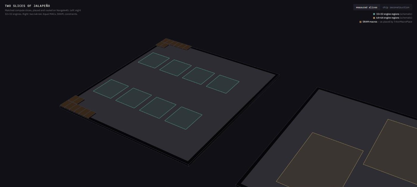
Added September 2026. Section 13 left open whether 32 beats 64, since that depended on wiring costs my tools could not see. I have since run the comparison through OpenROAD, the open-source place-and-route flow, on the Nangate45 library: real placement, routed wires and clock trees, with matched slices built to the same discipline as everything above. Eight 32x32 engines against two 64x64, with equal MACs, equal accumulators, equal SRAM macros, one shared operand port, and identical constraints and tool effort at every step.
The answer changed three times. Bare compute domains said fine granularity wins or ties everywhere, and the distributor cost I had worried about measured about 1% of area. Full slices with SRAM macros said the opposite: the coarse slice placed smaller, clocked 17 to 20% faster, and burned less power, because slice plumbing scales with engine count rather than engine width. Then I made the model match the chip zartbot describes, with the reduction pipelined into stages the way a real tensor unit is, and most of both prior results went away. Pipelined, the fine slice clocks about 10% faster and uses about 14% less power, the coarse slice keeps about a 3% area advantage, and cycle behavior is decided entirely by operand bandwidth: a tie below the feed knee, with fine ahead only when a slice gets more bytes per cycle than the public numbers say Jalapeño's slices get.
So the wiring costs exist, and they do not pick a winner. At the operand bandwidth the real chip runs, 32 and 64 are interchangeable in both layout and cycle count, which leaves 64x64 standing on the other reasons given above: fewer units to schedule, simpler tiling, easier yield harvesting, and a bandwidth budget that makes finer granularity pointless. The choice comes down to logistics. One more entry for the list in section 14: the unpipelined RTL comparison, like both cycle simulators before it, was biased, this time against whichever side buffered a large combinational adder tree worse.
The layouts are worth looking at: the placer puts all sixteen SRAM macros of the coarse slice into one corner and splits the fine slice's across two. Both placed dies, with their real macro coordinates, are in an interactive 3D viewer alongside a speculative full-chip reconstruction.
Sources
- zartbot, "Jalapeño architecture analysis": the teardown that most shaped this piece. ↩
- Tom's Hardware, Hot Chips 2026 coverage; OpenAI announcement. ↩
- ServeTheHome, "OpenAI Jalapeno Custom AI ASIC at Hot Chips 2026"; The Register. ↩